Piotr Wozniak, 1990
This text was taken from P.A.Wozniak, Optimization of learning, Master’s Thesis, University of Technology in Poznan, 1990 and adapted for publishing as an independent article on the web. (P.A.Wozniak, Sep 17, 1998)
Instead of improving the mathematical apparatus employed in the Algorithm SM-4, I decided to reshape the concept of modifying the function of optimum intervals.
Let us have a closer look at the major faults of the Algorithm SM-4 disregarding minor inefficiencies:
- In the course of repetition it may happen that one of the intervals will be calculated as shorter than the preceding one. This is certainly inconsistent with general assumptions leading to the SuperMemo method. Moreover, validity of such an outcome was refuted by the results of application of the Algorithm SM-5 (see further). This malfunction could be prevented by disallowing intervals to increase or drop beyond certain values, but such an approach would tremendously slow down the optimization process interlinking optimal intervals by superfluous dependencies. The discussed case was indeed observed in one of the databases. The discrepancy was not eliminated by the end of the period in which the Algorithm SM-4 was used despite the fact that the intervals in question were only two weeks long
- E-Factors of particular items are constantly modified (see Step 6 of the Algorithm SM-4 ) thus in the OI matrix an item can pass from one difficulty category to another. If the repetition number for that item is large enough, this will result in serious disturbances of the repetitory process of that item. Note that the higher the repetition number, the greater the difference between optimal intervals in neighboring E-Factor category columns. Thus if the E-Factor increases the optimal interval used for the item can be artificially long, while in the opposite situation the interval can be much too short
The Algorithm SM-4 tried to interrelate the length of the optimal interval with the repetition number. This approach seems to be incorrect because the memory is much more likely to be sensitive to the length of the previously applied inter-repetition interval than to the number of the repetition (previous interval is reflected in memory strength while the repetition number is certainly not coded – see Molecular model of memory comprising elements of the SuperMemo theory).
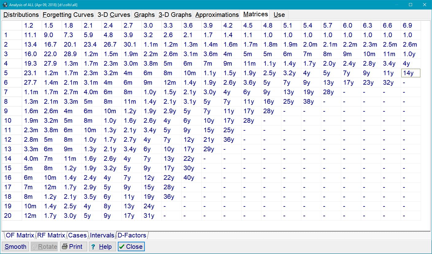
Because of the above reasons I decided to represent the function of optimal intervals by means of the matrix of optimal factors – OF matrix – rather than the OI matrix (see Fig. 3.3).
(Fig. 3.3)
The newly applied function of optimal intervals had the following form:
I(n,EF)=OF(n,EF)*I(n-1,EF)
I(1,EF)=OF(1,EF)
where:
I(n,EF) – the n-th inter-repetition interval for an item of a given E-Factor EF (in days)
OF(n,EF) – the entry of the OF matrix corresponding to the n-th repetition and the E-Factor EF
In accordance with previous observations the entries of the OF matrix were not allowed to drop below 1.2 (cf. the formulation of the Algorithm SM-2).
It is easy to notice that the application of the OF matrix eliminates both aforementioned shortcomings of the Algorithm SM-4:
- intervals cannot get shorter in subsequent repetition (each of them is at least 1.2 times as long as the preceding one),
- changing the E-Factor category increases the next applied interval only as many times as it is required by the corresponding entry of the OF matrix.
| The final formulation of the algorithm used in SuperMemo 5 is presented below (Algorithm SM-5):1. Split the knowledge into smallest possible items2. With all items associate an E-Factor equal to 2.53. Tabulate the OF matrix for various repetition numbers and E-Factor categories (see Fig. 3.3). Use the following formula:OF(1,EF):=4 for n>1 OF(n,EF):=EFwhere:OF(n,EF) – optimal factor corresponding to the n-th repetition and the E-Factor EF4. Use the OF matrix to determine inter-repetition intervals:I(n,EF)=OF(n,EF)*I(n-1,EF) I(1,EF)=OF(1,EF)where:I(n,EF) – the n-th inter-repetition interval for an item of a given E-Factor EF (in days) OF(n,EF) – the entry of the OF matrix corresponding to the n-th repetition and the E-Factor EF5. After each repetition assess the quality of repetition responses in the 0-5 grade scale (cf. Algorithm SM-2)6. After each repetition modify the E-Factor of the recently repeated item according to the formula:EF’:=EF+(0.1-(5-q)*(0.08+(5-q)*0.02))where:EF’ – new value of the E-Factor EF – old value of the E-Factor q – quality of the response in the 0-5 grade scale If EF is less than 1.3 then set EF to 1.37. After each repetition modify the relevant entry of the OF matrix. An exemplary formulas constructed arbitrarily and used in the modification could look like this (those used in the SuperMemo 5.3 are presented in Fig. 3.4):OF’:=OF*(0.72+q*0.07) OF”:=(1-fraction)*OF+fraction*OF’where:OF” – new value of the OF entry OF’ – auxiliary value of the OF entry used in calculations OF – old value of the OF entry fraction – any number between 0 and 1 (the greater it is the faster the changes of the OF matrix) q – quality of the response in the 0-5 grade scaleNote that for q=4 the OF does not change. It increases for q>4 and decreases for q<4. See the procedure presented in Fig. 5 to avoid the pitfalls of oversimplification8. If the quality response was lower than 3 then start repetitions for the item from the beginning without changing the E-Factor9. After each repetition session of a given day repeat again all items that scored below four in the quality assessment. Continue the repetitions until all of these items score at least four |
| Fig. 3.4 – The procedure used in the SuperMemo 5.3 for calculation of the new optimal factor after a repetition (simplified for the sake of clarity without significant change to the course of computation): |
| procedure calculate_new_optimal_factor;input:interval_used – the last interval used for the item in questionquality – the quality of the repetition responseused_of – the optimal factor used in calculation of the last interval used for the item in questionold_of – the previous value of the OF entry corresponding to the relevant repetition number and the E-Factor of the itemfraction – a number belonging to the range (0,1) determining the rate of modifications (the greater it is the faster the changes of the OF matrix)output:new_of – the newly calculated value of the considered entry of the OF matrixlocal variables:modifier – the number determining how many times the OF value will increase or decreasemod5 – the value proposed for the modifier in case of q=5mod2 – the value proposed for the modifier in case of q=2beginmod5:=(interval_used+1)/interval_used; if mod5<1.05 then mod5:=1.05; mod2:=(interval_used-1)/interval_used; if mod2>0.75 then mod2:=0.75; if quality>4 then modifier:=1+(mod5-1)*(quality-4) else modifier:=1-(1-mod2)/2*(4-quality); if modifier<0.05 then modifier:=0.05; new_of:=used_of*modifier; if quality>4 then if new_of<old_of then new_of:=old_of; if quality<4 then if new_of>old_of then new_of:=old_of; new_of:=new_of*fraction+old_of*(1-fraction); if new_of<1.2 then new_of:=1.2;end; |
3.5. Random dispersal of optimal intervals
To improve the optimization process further, a mechanism was introduced that may seem to contradict the principle of optimal repetition spacing. Let us reconsider a significant fault of the Algorithm SM-5: A modification of an optimal factor can be verified for its correctness only after the following conditions are met:
- the modified factor is used in calculation of an inter-repetition interval
- the calculated interval elapses and a repetition is done yielding the response quality which possibly indicates the need to increase or decrease the optimal factor
This means that even a great number of instances used in modification of an optimal factor will not change it significantly until the newly calculated value is used in determination of new intervals and verified after their elapse.
The process of verification of modified optimal factors after the period necessary to apply them in repetitions will later be called the modification-verification cycle. The greater the repetition number the longer the modification-verification cycle and the greater the slow-down in the optimization process.
To illustrate the problem of modification constraint let us consider calculations from Fig. 3.4.
One can easily conclude that for the variable INTERVAL_USED greater than 20 the value of MOD5 will be equal 1.05 if the QUALITY equals 5. As the QUALITY=5, the MODIFIER will equal MOD5, i.e. 1.05. Hence the newly proposed value of the optimal factor (NEW_OF) can only be 5% greater than the previous one (NEW_OF:=USED_OF*MODIFIER). Therefore the modified optimal factor will never reach beyond the 5% limit unless the USED_OF increases, which is equivalent to applying the modified optimal factor in calculation of inter-repetition intervals.
Bearing these facts in mind I decided to let inter-repetition intervals differ from the optimal ones in certain cases to circumvent the constraint imposed by a modification-verification cycle.
I will call the process of random modification of optimal intervals dispersal.
If a little fraction of intervals is allowed to be shorter or longer than it should follow from the OF matrix then these deviant intervals can accelerate the changes of optimal factors by letting them drop or increase beyond the limits of the mechanism presented in Fig. 3.4. In other words, when the value of an optimal factor is much different from the desired one then its accidental change caused by deviant intervals shall not be leveled by the stream of standard repetitions because the response qualities will rather promote the change than act against it.
Another advantage of using intervals distributed round the optimal ones is elimination of a problem which often was a matter of complaints voiced by SuperMemo users – the lumpiness of repetition schedule. By the lumpiness of repetition schedule I mean accumulation of repetitory work in certain days while neighboring days remain relatively unburdened. This is caused by the fact that students often memorize a great number of items in a single session and these items tend to stick together in the following months being separated only on the base of their E-Factors.
Dispersal of intervals round the optimal ones eliminates the problem of lumpiness. Let us now consider formulas that were applied by the latest SuperMemo software in dispersal of intervals in proximity of the optimal value. Inter-repetition intervals that are slightly different from those which are considered optimal (according to the OF matrix) will be called near-optimal intervals. The near-optimal intervals will be calculated according to the following formula:
NOI=PI+(OI-PI)*(1+m)
where:
NOI – near-optimal interval
PI – previous interval used
OI – optimal interval calculated from the OF matrix (cf. Algorithm SM-5)
m – a number belonging to the range <-0.5,0.5> (see below)
or using the OF value:
NOI=PI*(1+(OF-1)*(1+m))
The modifier m will determine the degree of deviation from the optimal interval (maximum deviation for m=-0.5 or m=0.5 values and no deviation at all for m=0).
In order to find a compromise between accelerated optimization and elimination of lumpiness on one hand (both require strongly dispersed repetition spacing) and the high retention on the other (strict application of optimal intervals required) the modifier m should have a near-zero value in most cases.
The following formulas were used to determine the distribution function of the modifier m:
- the probability of choosing a modifier in the range <0,0.5> should equal 0.5:
integral from 0 to 0.5 of f(x)dx = 0.5
- the probability of choosing a modifier m=0 was assumed to be hundred times greater than the probability of choosing m=0.5:
f(0)/f(0.5)=100
- the probability density function was assumed to have a negative exponential form with parameters a and b to be found on the base of the two previous equations:
f=a*exp(-b*x)
The above formulas yield values a=0.04652 and b=0.09210 for m expressed in percent.
From the distribution function
itegral from -m to m of a*exp(-b*abs(x))dx = P (P denotes probability)
we can obtain the value of the modifier m (for m>=0):
m=-ln(1-b/a*P)/b
Thus the final procedure to calculate the near-optimal interval looks like this:
a:=0.047;
b:=0.092;
p:=random-0.5;
m:=-1/b*ln(1-b/a*abs(p));
m:=m*sgn(p);
NOI:=PI*(1+(OF-1)*(100+m)/100);
where:
random – function yielding values from the range <0,1) with a uniform distribution of probability
NOI – near-optimal interval
PI – previously used interval
OF – pertinent entry of the OF matrix
3.6. Improving the predetermined matrix of optimal factors
The optimization procedures applied in transformations of the OF matrix appeared to be satisfactorily efficient resulting in fast convergence of the OF entries to their final values.
However, in the period considered (Oct 17, 1989 – May 23, 1990) only those optimal factors which were characterized by short modification-verification cycles (less than 3-4 months) seem to have reached their equilibrial values.
It will take few further years before more sound conclusions can be drawn regarding the ultimate shape of the OF matrix. The most interesting fact apparent after analyzing 7-month-old OF matrices is that the first inter-repetition interval should be as long as 5 days for E-Factor equal 2.5 and even 8 days for E-Factor equal 1.3! For the second interval the corresponding values were about 3 and 2 weeks respectively.
The newly-obtained function of optimal intervals could be formulated as follows:
I(1)=8-(EF-1.3)/(2.5-1.3)*3
I(2)=13+(EF-1.3)/(2.5-1.3)*8
for i>2 I(i)=I(i-1)*(EF-0.1)
where:
I(i) – interval after the i-th repetition (in days)
EF – E-Factor of the considered item.
To accelerate the optimization process, this new function should be used to determine the initial state of the OF matrix (Step 3 of the SM-5 algorithm). Except for the first interval, this new function does not differ significantly from the one employed in Algorithms SM-0 through SM-5. One could attribute this fact to inefficiencies of the optimization procedures which, after all, are prejudiced by the fact of applying a predetermined OF matrix. To make sure that it is not the fact, I asked three of my colleagues to use experimental versions of the SuperMemo 5.3 in which univalent OF matrices were used (all entries equal to 1.5 in two experiments and 2.0 in the remaining experiment).
Although the experimental databases have been in use for only 2-4 months, the OF matrices seem to slowly converge to the form obtained with the use of the predetermined OF matrix. However, the predetermined OF matrices inherit the artificial correlation between E-Factors and the values of OF entries in the relevant E-Factor category (i.e. for n>3 the value OF(n,EF) is close to EF). This phenomenon does not appear in univalent matrices which tend to adjust the OF matrices more closely to requirements posed by such arbitrarily chosen elements of the algorithm as initial value of E-Factors (always 2.5), function modifying E-Factors after repetitions etc.
3.7. Propagation of changes across the matrix of optimal factors
Having noticed the earlier mentioned regularities in relationships between entries of the OF matrix I decided to accelerate the optimization process by propagation of modifications across the matrix. If an optimal factor increases or decreases then we could conclude that the OF factor that corresponds to the higher repetition number should also increase.
This follows from the relationship OF(i,EF)=OF(i+1,EF), which is roughly valid for all E-Factors and i>2. Similarly, we can consider desirable changes of factors if we remember that for i>2 we have OF(i,EF’)=OF(i,EF”)*EF’/EF” (esp. if EF’ and EF” are close enough). I used the propagation of changes only across the OF matrix that had not yet been modified by repetition feed-back. This proved particularly successful in case of univalent OF matrices applied in the experimental versions of SuperMemo mentioned in the previous paragraph.
The proposed propagation scheme can be summarized as this:
1. After executing Step 7 of the Algorithm SM-5 locate all neighboring entries of the OF matrix that has not yet been modified in the course of repetitions, i.e. entries that did not enter the modification-verification cycle. Neighboring entries are understood here as those that correspond to the repetition number +/- 1 and the E-Factor category +/- 1 (i.e. E-Factor +/- 0.1)
2. Modify the neighboring entries whenever one of the following relations does not hold:
- for i>2 OF(i,EF)=OF(i+1,EF) for all EFs
- for i>2 OF(i,EF’)=OF(i,EF”)*EF’/EF”
- for i=1 OF(i,EF’)=OF(i,EF”)
The selected relation should hold as the result of the modification
3. For all the entries modified in Step 2 repeat the whole procedure locating their yet unmodified neighbors.
Propagation of changes seems to be inevitable if one remembers that the function of optimal intervals depends on such parameters as:
- student’s capacity
- student’s self-assessment habits (the response quality is given according to the student’s subjective opinion)
- character of the memorized knowledge etc.
Therefore it is impossible to provide an ideal, predetermined OF matrix that would dispense with the use of the modification-verification process and, to a lesser degree, propagation schemes
3.8. Evaluation of the Algorithm SM-5
The Algorithm SM-5 has been in use since October 17, 1989 and has surpassed all expectations in providing an efficient method of determining the desired function of optimal intervals, and in consequence, improving the acquisition rate (15,000 items learnt within 9 months). Fig. 3.5 indicates that the acquisition rate was at least twice as high as that indicated by combined application of the SM-2 and SM-4 algorithms!
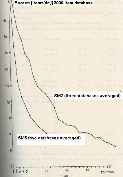
(Fig. 3.5)
The knowledge retention increased to about 96% for 10-month-old databases. Below, some knowledge retention data in selected databases are listed to show the comparison between the SM-2 and SM-5 algorithms:
Date – date of the measurement,
Database – name of the database; ALL means all databases averaged
Interval – average current interval used by items in the database
Retention – knowledge retention in the database
Version – version of the algorithm applied to the database
| Date | Database | Interval | Retention | Version |
| Dec 88 | EVD | 17 days | 81% | SM-2 |
| Dec 89 | EVG | 19 days | 82% | SM-5 |
| Dec 88 | EVC | 41 days | 95% | SM-2 |
| Dec 89 | EVF | 47 days | 95% | SM-5 |
| Dec 88 | all | 86 days | 89% | SM-2 |
| Dec 89 | all | 190 days | 92% | SM-2, SM-4 and SM5 |
In the process of repetition the following distribution of response qualities was recorded:
| Quality | Fraction |
| 0 | 0% |
| 1 | 0% |
| 2 | 11% |
| 3 | 18% |
| 4 | 26% |
| 5 | 45% |
This distribution, in accordance to the assumptions underlying the Algorithm SM-5 , yields the average response quality equal 4. The forgetting index equals 11% (items with quality lower than 3 are regarded as forgotten). Note, that the retention data indicate that only 4% of items in a database are not remembered. Therefore forgetting index exceeds the percentage of forgotten items 2.7 times.
In a 7-month old database, it was found that 70% of items had not been forgotten even once in the course of repetitions preceding the measurement, while only 2% of items had been forgotten more than 3 times. Concerning the convergence of the algorithm modifying the function of optimal intervals, it is too early for a conclusive assessment (see Fig. 3.6).
(Fig. 3.6)
Fig. 3.6. Changes in the OF matrix for entries characterized by a short modification-verification cycle
In Chapter 4 the following statistical data pertaining to an 8-month-old SuperMemo process can be found:
- distribution of E-Factors
- distribution of current intervals
- matrix of optimal factors
- equivalent of the matrix of optimal intervals (calculated on the base of the OF matrix)